Query Execution Study Note

Query execution is part of the query processor. The SQL query will be firstly compiled then be executed. A simple diagram shows clearly below.

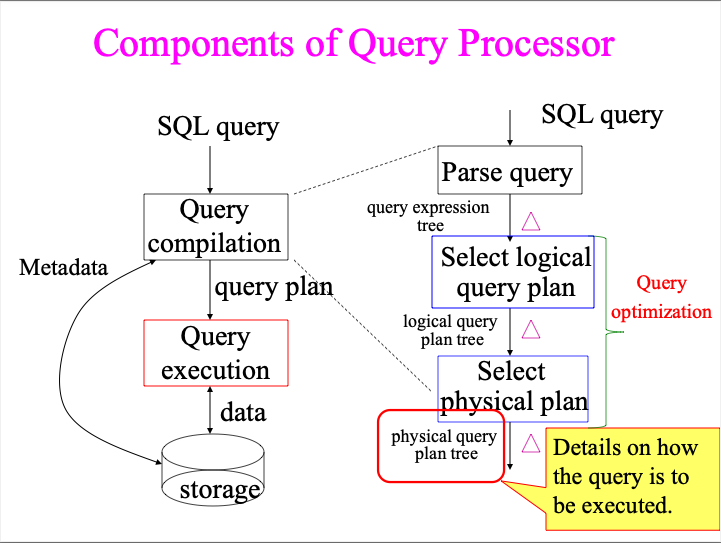
Figure 1: Components of Query Processor [PNG]

This note is mainly on query execution.

Table of Contents
Cost Model
Classification of Physical Operators

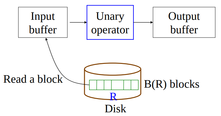
Cost Model

Why? And Some Assumptions

Important in query optimization
Here we consider I/O cost only
We assume operands are relations stored on disk, but operator results will be left in main memory (e.g., pipelined to next operator in query plan)
So we don’t include the cost of writing the result

We will also need some notations, aka, cost parameters.

Cost parameters

$M$ = number of blocks/pages that are available in main memory
$B(R)$ = number of blocks holding $R$
$T(R)$ = number of tuples in $R$
$V(R,a)$ = number of distinct values of the attribute $a$ of $R$

Two Types of Scanning Tables

Clustered

The table is clustered (i.e., block consists only of records from this table)

# of I/O’s = # of blocks

Unclustered

The table is unclustered (e.g. its records are placed in blocks with those of other tables)

May need one block read for each record

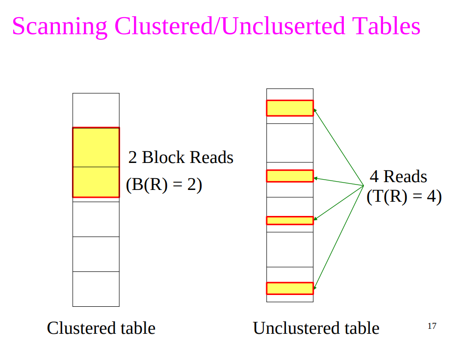
Figure 2: Scanning Clustered/Uncluserted Tables [PNG]

Cost of the Scan Operator

Clsutered relation

We assume clustered relations to estimate the costs of other physical operators.
Table scan: $B(R)$

Unclustered relation

Table scan: $T(R)$

Classification of Physical Operators

One-pass Algorithms

Selection, $\sigma(R)$ and Projection, $\Pi(R)$

Both are tuple-at-a-time algorithms
Cost: $B(R)$

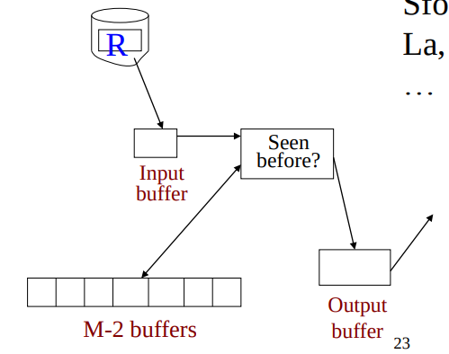
Figure 3: Selection and projection diagram [PNG]

Duplicate elimination, $\delta(R)$

Assumption: $B(\delta(R)) \le M-2$, or roughly $M$
It needs to keep a dictionary in memory
- Balanced Search Tree (BST)
- Hash Table
- Etc.
Cost: $B(R)$

Figure 4: Duplicate elimination diagram [PNG]

Grouping, $\gamma_{\text{city, sum(price)}}(R)$

Assumption: number of cities and sums fit in memory
It also needs to keep a dictionary in memory
- In addition, it also stores the sum(price) for each city
Cost: $B(R)$

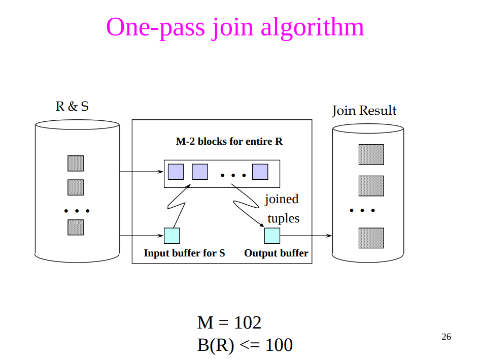
Binary operations, $R\cap S, R\cup S, R-S, R\bowtie S$

Assumption: $\text{min}(B(R), B(S)) \le M-2$, or roughly M
Scan a smaller table of R and S into main memory, then read the other one, block by block
Cost: $B(R)+B(S)$, assume both are clustered
Example: $R\cap S$
- Assumption: set-based, no duplicates
- Read $S$ into $M-2$ buffers and build a search structure
- Read each block of $R$, and for each tuple $t$ of $R$, see if $t$ is also in $S$
- If so, copy $t$ to the output; if not, ignore $t$

Figure 5: One-pass join algorithm diagram [PNG]

Nested-Loop Join Algorithms

Tuple-based Nested Loop Joins

$R\bowtie S$
Assumption: Neither relation is clustered

Pseudo-Python-Code

for r in R: # r is a tuple in R
  for s in S: # s is a tuple in S
    if canBeJoined(r,s):
      return (r,s)

Cost: $T(R)T(S)$

Block-based Nested Loop Joins

$R\bowtie S$
- $R$ is the outer relation, $S$ is the inner relation
Assumption
- Both relation are clustered
- $B(R) \le B(S)$ and $B(S) > M$

Pseudo-Python-Code

for br in R: # (M-2) blocks of br
  for bs in S:
    for r in br: # r is a tuple in R
      for s in bs: # s is a tuple in S
        if canBeJoined(r,s):
          return (r,s)

Cost ($M\ge 3$ in order for $M-2\ge 1$)
- If R is the outer relation $$ B(R)+\frac{B(R)B(S)}{M-2} $$ where $B(R)$ is the cost of reading $R$ once, $\frac{B(R)}{M-2}$ is the number of outer loop runs. Each run needs to read $S$, so the latter is multiplied by $B(S)$.
- If S is the outer relation $$ B(S)+\frac{B(R)B(S)}{M-2} $$
Takeaway: It is better to iterate over the smaller relation first

Two-pass Algorithms Based on Sorting

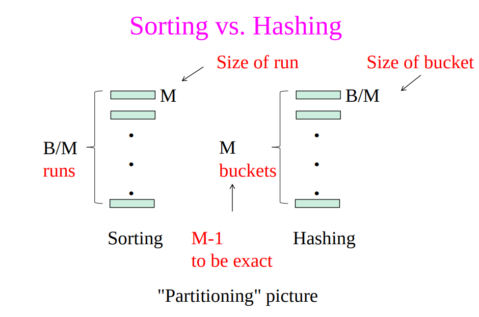
Sort-based vs. Hash-based Algorithms

Sort-based algorithms sometimes allow us to produce a result in sorted order and take advantage of that sort later
Hash-based algorithms for binary operations have a size requirement only on the smaller of two input relations
Hash-based algorithm depends on the buckets being of equal size, which may not be true if data are skewed

Duplicate Elimination $\delta(R)$ Based on Sorting

Idea: Sort first, then eliminate duplicates
Assumption: $B(R) \le M^2$ (roughly)
- $B(R)/M$ is # of runs
- # of runs has to be smaller than or equal to $M-1$ to complete the merging in the second pass
- Therefore, $B(R)/M \le M-1$
Steps
- Pass 1: sort runs of size $M$ and then write
  - Cost: $2B(R)$
- Pass 2: merge $M-1$ runs, but include each tuple only once
  - Cost: $B(R)$
Cost: $3B(R)$

Grouping $\gamma_{\text{city, sum(price)}}(R)$ Based on Sorting

Assumption: $B(R) \le M^2$
Steps
- Pass 1: sort runs of size $M$ and then write
  - Cost: $2B(R)$
- Pass 2: merge $M-1$ runs, but include each tuple only once. Also, compute sum(price) for group during the merge phase (new compared to duplicate elimination based on sorting)
  - Cost: $B(R)$
Cost: $3B(R)$

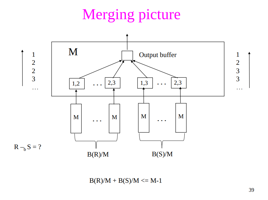
Binary operations $R\cap S, R\cup S, R-S$ Based on Sorting

Note that join operator ($\bowtie$) is not included this time. Why? Because there are a large number of tuples with the same value on the join attribute(s), however the buffer can not hold all joining tuples (with the same value on join attribute) for at least one relation.

Idea: Sort $R$, sort $S$, then do their binary operations
Assumption: $B(R)+B(S) \le M^2$ (roughly)
Steps
- Pass 1: Split $R$ into runs of size $M$, then split $S$ into runs of size $M$
  - Cost: $2B(R)+2B(S)$
- Pass 2: Merge $M-1$ runs from $R$ and $S$, then output a tuple on a case by cases basis
  - Cost: $B(R)$
Cost: $3B(R)+3B(S)$

Sort-Merge Join

Assumption:
- The buffer is enough to hold join tuples for at least one relation
  - Note that the buffer also needs to hold a block for each run of the other relation
- $B(R)+B(S) \le M^2$ (roughly)
Cost: $3B(R)+3B(S)$

Simple Sort-based Join

Idea: Sort $R$, sort $S$, then do their binary operations
Assumption: $B(R)\le M^2$, $B(S)\le M^2$, and at least one set of the tuples with a common value for the join attributes fit in $M$ (or $M-2$ to be exact)
- Note that we only need one page buffer for the other relation
Steps
- Step 1: Start by completely sorting both $R$ and $S$ on the join attribute (assuming this can be done in 2 passes):
  - Cost: $4B(R)+4B(S)$, because we need to write result to disk
- Step 2: Read both relations in sorted order, match tuples
  - Cost: $B(R)+B(S)$
Cost: $5B(R)+5B(S)$
Note
- Can use as many buffers as possible to load join tuples from one relation (with the same join value), say $R$
  - Only one buffer is needed for the other relation, say $S$
- If we still can not fit all join tuples from $R$
  - Need to use nested loop algorithm, higher cost

Two-pass Algorithms Based on Hashing

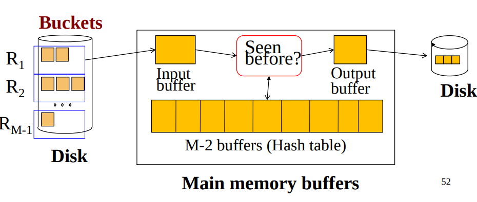
Duplicate Elimination $\delta(R)$ Based on Hashing

Idea
- Partition a relation R into buckets on disk. Each bucket has size approximately $B(R)/M$
- Does each bucket fit in main memory?
  - Yes if $B(R)/(M-1) \le M-2$ (i.e., approx. $B(R) \le M^2$)
- Apply the one-pass duplicate elimination $\delta$ algorithm for each $R_i$
Assumption: $B(R) \le M^2$ (roughly)
- Exact: $B(R)/(M-1) \le M-2$
Steps
- Step 1: Partition $R$ into $M-1$ buckets
- Step 2: Apply $\delta$ to each bucket (must read it into main memory)
Cost: $3B(R)$

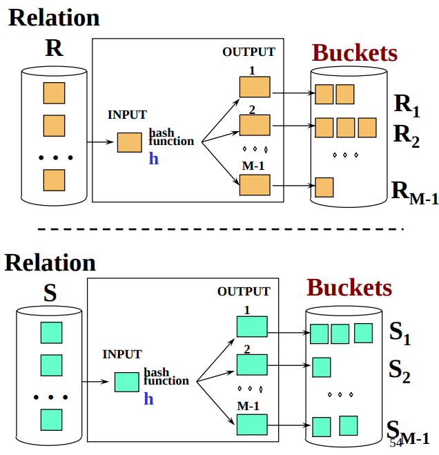
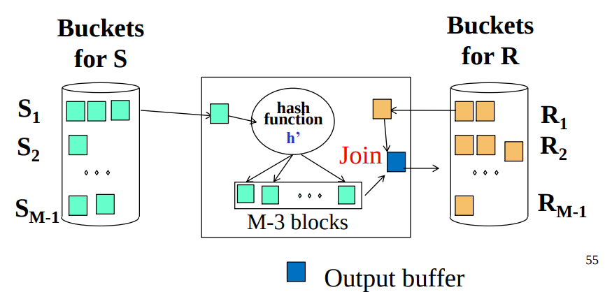
Figure 8: Two-pass Duplicate Elimination Diagram Based on Hashing [PNG]

Partitioned Hash-Join

Assumption: $\text{min}(B(R),B(S)) \le M^2$
- Exact: $\frac{\text{min}(B(R),B(S))}{M-1} \le M-3$
- If we don’t use hash table to speed up the lookup: $\frac{\text{min}(B(R),B(S))}{M-1} \le M-2$
Steps
- Step 1
  - Hash $S$ into $M$ - 1 bucket
  - Send all buckets to disk
- Step 2
  - Hash $R$ into $M$ - 1 bucket
  - Send all buckets to disk
- Step 3
  - Join every pair of corresponding buckets
Cost: $3B(R)+3B(S)$

Figure 10: Partitioned Hash-Join Pass 2 (Steps 3) Diagram [PNG]

Index-Based Algorithms

The existence of an index on one ore more attributes of a relation makes available some algorithms that would not be feasible without the index • Useful for selection operations • Also, algorithms for join and other binary operations use indexes to good advantage

Index-Based Selection, $\sigma_{a=v}(R)$

Assumption: We here ignored the cost of reading index blocks
Cost
- Clustered index on attribute $a$: $B(R)/V(R,a)$
- Unclustered index on attribute $a$: $T(R)/V(R,a)$

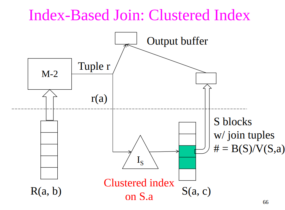
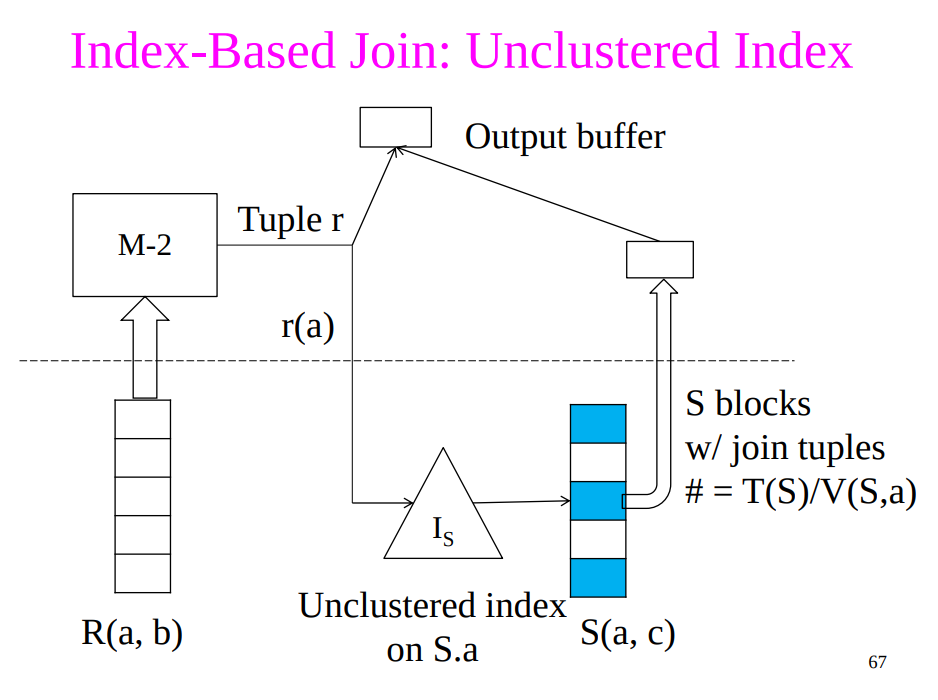
Index-Based Join, $R\bowtie S$

Assumption: Assume $S$ has an index on the join attribute
Steps
- Iterate over $R$, for each tuple, fetch corresponding tuple $s$ from $S$
Cost
- Clustered index $$B(R) + \frac{T(R)B(S)}{V(S,a)}$$
- Unclustered index $$B(R) + \frac{T(R)T(S)}{V(S,a)}$$
Indexed-Based Join vs NLJ
- Recall the cost for Nested Loop Join (NLJ), assume both $R$ and $S$ are clustered $$B(R) + \frac{B(R)B(S)}{M-2}$$
- Index-Based wins NLJ if:
  - $$\frac{T(R)}{V(S,a)} < \frac{B(R)}{M-2}$$, or
  - $$V(S,a) > (M-2) \cdot \frac{T(R)}{B(R)}$$

Figure 11: Index-Based Join: Clustered Index Diagram [PNG]

Figure 12: Index-Based Join: Unclustered Index Diagram [PNG]

Index-Based Join with Two Indices

Assumption: Assume both $R$ and $S$ have a clustered index (e.g., B+-tree) on the join attribute
Then can perform a sort-merge join where sorting is already done (for free)
Cost: $B(R) + B(S)$

Table of Contents